Introduction: Standard Deviation Doesn’t Tell the Whole Story
Many data practitioners resort to the same summary statistics.
- Mean
- Variance
- Standard Deviation
But relying solely on standard deviation can hide important characteristics of data.
Two datasets may have identical means, identical standard deviations, and radically different behavior.
One may contain extreme outliers, whereas another may have unstable variation relative to its scale. A third may have small errors, but frequent deviations from expected behavior. This is where three often underused statistics become powerful.
- Mean Absolute Deviation (MAD) -> measures average deviation intuitively.
- Coefficient of Variation (CV) -> compares variability across scales.
- Kurtosis -> detects tail risk and outlier structure.
These metrics mainly appear in:
- algorithm diagnostics
- financial modeling
- anomaly detection
- manufacturing reliability
- feature engineering
- A/B testing
And they often reveal patterns standard deviation misses.
1. Mean Absolute Deviation: Variability Humans Can Interpret
Mean Absolute Deviation measures the average distance between each data point and the mean.
It tells us:
- How spread out the data is.
- How much observations deviate from the average.
- The consistency of data values.
$$MAD = \frac{\sum |x_i – \bar{x}|}{n}$$
Where:
xᵢ: Each individual data point.
x̄: The mean (average) of the dataset.
n: Total number of data points.
Practical Problem: Model Accuracy
Consider the predicted model accuracy of (78, 84, 94, 82, 72) (out of 100)
Step 1: Find Mean
$$\bar{x} = \frac{78 + 84 + 94 + 82 + 72}{5} = \frac{410}{5} = 82$$
Step 2: Compute Absolute Deviation
| Score | Deviation | Absolute Deviation |
|---|---|---|
| 78 | 78 - 82 = -4 | 4 |
| 84 | 84 - 82 = 2 | 2 |
| 94 | 94 - 82 = -10 | 12 |
| 82 | 82 - 82 = 2 | 0 |
| 72 | 72 - 82 = -12 | 10 |
Step 3: Calculate MAD
$$\frac{4 + 0 + 10 + 2 + 12}{5} = \frac{28}{5} = 5.6$$
This means that, on average, the model’s accuracy varies by 5.6 percentage points from the mean.
Why MAD Matters in Data Science
Applications:
- Forecast error analysis
- Model performance evaluation
- Outlier-resistant variability measurement
- Financial risk estimation
Unlike standard deviation, MAD is easier to interpret because it uses absolute values instead of squared distances.
If we consider an example of a sensor system, Low MAD indicates a stable measurement, whereas high MAD indicates a noisy sensor.
Coefficient of Variation: When Standard Deviation Misleads
The Coefficient of Variation (CV) is a measure of relative variability. It shows how much the data varies in relation to the mean.
A high CV means data points are more spread out (less consistent), whereas a low CV means data points are less spread out (more consistent).
$$CV = \frac{\sigma}{\mu} \times 100$$
Variable Definitions
\( CV \) = Coefficient of Variation
\( \sigma \) = Standard Deviation
\( \mu \) = Mean
Practical Problem: Comparing Two Machines
Suppose two machines produce bolts:
Machine A: {20,22,18,21,19}, Machine B: {100,110,90,105,95}
Step 1: Find the mean
Machine A: μ_A=20
Machine B: μ_B=100
Step 2: Standard Deviations
Using:
$$\sigma = \sqrt{\frac{\sum (x_i – \mu)^2}{n}}$$
For both machines:
$$\sigma = 1.41 \text{ for A}$$
$$\sigma = 7.07 \text{ for B}$$
Step 3: Compute CV
Machine A:
$$CV_A = \frac{1.41}{20} \times 100 = 7.05\%$$
Machine B:
$$CV_B = \frac{7.07}{100} \times 100 = 7.07\%$$
Both machines have nearly identical relative variability. Even though Machine B has a larger absolute spread, its variation relative to its mean is similar.
Applications of Coefficient of Variance (CV)
Used in:
- Comparing investment risk
- Manufacturing quality control
- Feature stability analysis
- Comparing datasets with different units
Example:
Comparing salary volatility and stock returns.
Where CV Matters in Data Science
A feature with high CV is unreliable. Imagine a sensor with a CV of 5 and another with a CV of 35. Here, the one with a CV of 5 is stable, whereas the other with 3 is unstable.
CV is unreliable when:
- Mean is near zero
- Mean is negative
- Ratio scales are violated
CV should only be used for ratio-scale data with meaningful zero (e.g., weight, income, response time), not interval scales like temperature in Celsius.
Kurtosis: Detecting Tail Risk Standard Metrics Miss
Kurtosis is a statistical measure that describes the shape of a distribution.
While often described as peakedness, kurtosis is more accurately a measure of tail heaviness and propensity for extreme observations.
It tells us whether data have:
- Heavy tails(more extreme values/outliers)
- Light tails(fewer extreme values)
- A normal-shaped distribution
In simple terms, kurtosis measures how prone a dataset is to extreme values. Higher kurtosis means a greater chance of unusual observations.
$$\text{Kurtosis} = \frac{\mu_4}{\sigma^4}$$
Variable Definitions
\( \mu_4 \) = The fourth central moment of the distribution
\( \sigma^4 \) = The standard deviation raised to the fourth power (variance squared)
Why This Matters
Kurtosis matters because two datasets can have equal variance. One can contain rare catastrophic events, whereas the other can be benign. Variance cannot distinguish them but kurtosis can.
Example: Fraud Detection
Transaction amounts:
Dataset A: {45,50,55,60,48}
Dataset B: {45,50,55,60,4000}
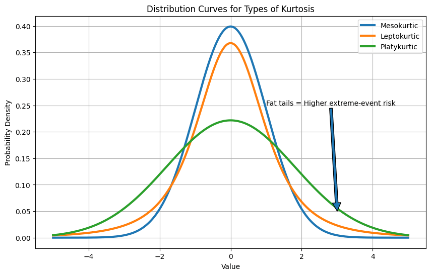
Types of Kurtosis
Same typical behavior, but dataset B has fat tails, and that’s likely an anomaly. High kurtosis exposes that.
Mesokurtic
A mesokurtic distribution has a moderate peak and tail thickness similar to a normal distribution. It has a normal level of outliers, and its kurtosis is equal to 3 (or excess kurtosis = 0).
Leptokurtic
A leptokurtic distribution has a sharper peak and heavier tails than a normal distribution. It indicates a higher probability of extreme values or outliers. Its kurtosis is greater than 3 (or excess kurtosis > 0).
Platykurtic
A platykurtic distribution has a flatter peak and lighter tails than a normal distribution. It indicates fewer extreme values or outliers. Its kurtosis is less than 3 (or excess kurtosis < 0).
Comparison between the Metrics
| Metric | Captures | Strength | Weakness |
|---|---|---|---|
| Standard Deviation | Squared spread | Common, powerful | Sensitive to outliers |
| MAD | Average deviation | Intuitive, robust | Less sensitive to extremes |
| CV | Relative variability | Compares scales | Breaks near zero mean |
| Kurtosis | Tail risk | Detects extreme events | Can be unstable in small samples |
Python Implementation
					import numpy as np
from scipy.stats import kurtosis

x = np.array([78,84,94,82,72])

mad = np.mean(abs(x - np.mean(x)))
cv = np.std(x)/np.mean(x)*100
kurt = kurtosis(x, fisher=False)

print(mad, cv, kurt)