When people talk about machine learning, they usually focus on neural networks, deep learning, or massive datasets. But underneath many machine learning algorithms lies something much more fundamental: linear algebra.
One of the most powerful techniques in linear algebra is LU decomposition. Even though most developers use machine learning libraries that handle the math automatically, LU decomposition is quietly working behind the scenes to make many computations faster and more stable.
In this article, we will explore:
- What LU decomposition actually is
- Why machine learning systems use it
- The mathematics behind it
- A real-world regression example
- Why LU decomposition is often better than matrix inversion
- Applications in modern machine learning
What is LU Decomposition?
LU decomposition is a technique used to break a large matrix into two simpler matrices.
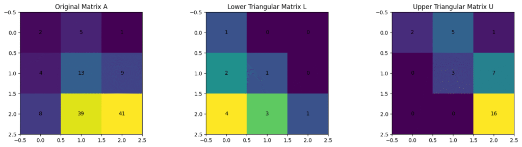
Suppose we have an original matrix:
$$A = \begin{bmatrix} 2 & 5 & 1 \\ 4 & 13 & 9 \\ 8 & 39 & 41 \end{bmatrix}$$
LU decomposition factorizes this matrix into:
$$A = LU$$
where:
$$L = \begin{bmatrix} 1 & 0 & 0 \\ 2 & 1 & 0 \\ 4 & 3 & 1 \end{bmatrix}, \quad U = \begin{bmatrix} 2 & 5 & 1 \\ 0 & 3 & 7 \\ 0 & 0 & 16 \end{bmatrix}$$
Gaussian elimination is used to decompose a matrix into A = LU.
That is the entire idea behind LU decomposition:
Instead of solving problems using one complicated matrix, we split it into two simpler triangular matrices that are easier for computers to work with.
Why is LU Decomposition Important?
In machine learning, many algorithms eventually reduce to solving equations like:
$$Ax = b$$
This appears in:
- Linear Regression
- Least Squares Problems
- Gaussian Processes
- Kalman Filters
- Optimization systems
- Numerical simulations
A beginner might try solving this using matrix inversion:
$$x = A^{-1}b$$
But in practice, directly computing matrix inverses is slow and numerically unstable. LU decomposition avoids this problem. Instead of inverting the matrix, we decompose it:
$$A = LU$$
Then solve the problem in two easier steps.
The Core Mathematical Idea
Suppose: $$Ax = b$$
If: $$A = LU$$
then: $$LUx=b$$
Now let: $$Ux=y$$
So the problem becomes:
- Solve: $$Ly=b$$
- Then solve: $$Ux=y$$
- Because both L and U are triangular matrices, solving them becomes computationally efficient.
- This is one reason why LU decomposition is heavily used in scientific computing and machine learning systems.
LU decomposition is essentially a way of converting a difficult global problem into smaller local problems. Instead of attacking the matrix all at once, we simplify it step-by-step using elimination. In many ways, this mirrors how optimization itself works in machine learning: breaking complexity into manageable computations.
LU Decomposition in Linear Regression
Linear regression tries to fit the best line through data points.
The equation is: $$y = \theta_0 + \theta_1 x$$
Using matrices: $$Xθ = y$$
The normal equation becomes: $$(X^T X)\theta = X^T y$$
Many tutorials directly compute: $$\theta = (X^T X)^{-1} X^T y$$
But this is not always the best approach. Instead, machine learning libraries often solve: $$(X^T X)\theta = X^T y$$
using decomposition methods like LU decomposition. This improves both efficiency and numerical stability.
Real-World Example: Predicting House Prices
Suppose we have the following dataset:
$$House Size (sq.ft): 1000, 1500, 2000$$
$$Price ($1000): 200, 300, 400$$
We create the design matrix:
$$X = \begin{bmatrix} 1 & 1000 \\ 1 & 1500 \\ 1 & 2000 \end{bmatrix}$$
And target vector:
$$y = \begin{bmatrix} 200 \\ 300 \\ 400 \end{bmatrix}$$
Now compute: $$X^T X = \begin{bmatrix} 3 & 4500 \\ 4500 & 7250000 \end{bmatrix}$$
And: $$X^T y = \begin{bmatrix} 900 \\ 1450000 \end{bmatrix}$$
Now we solve: $$(X^T X)\theta = X^T y$$
using LU decomposition.
Step-by-Step LU Decomposition
Let the original matrix be:
$$A = \begin{bmatrix} 3 & 4500 \\ 4500 & 7250000 \end{bmatrix}$$
We decompose it into: $$A = LU$$
Where: $$Ux = y$$
Final result:
$$\begin{aligned}
\theta_0 &= 0 \\
\theta_1 &= 0.2
\end{aligned}$$
So the regression equation becomes: $$\text{Price} = 0.2 \times \text{House Size}$$
This means every additional square foot increases the predicted house price by approximately 200.
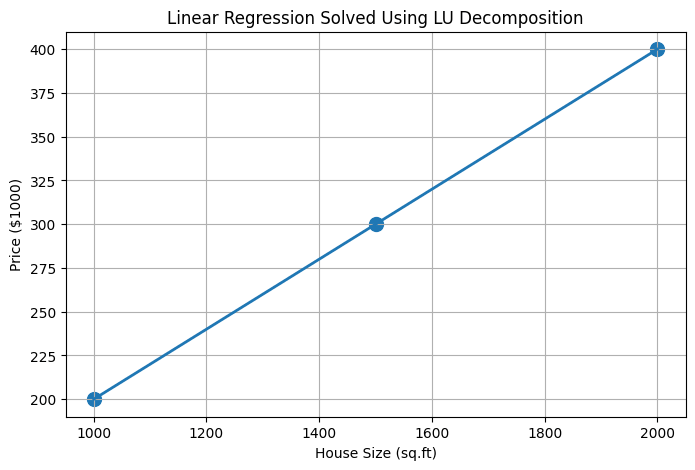
This graph illustrates a linear regression model for predicting house prices based on house size. The regression line is obtained by solving the normal equations using LU decomposition, demonstrating how matrix factorization can efficiently compute machine learning model parameters.
Why Not Use Matrix Inversion?
When first learning linear regression, it is easy to assume that matrix inversion is the standard way to solve everything. But in practical machine learning systems, direct inversion is usually avoided.
Here is why.
1. Matrix Inversion is Expensive
Computing inverses for large matrices requires significant computation. Its complexity is roughly: $$O(n^3)$$
As datasets grow, this becomes inefficient.
2. Numerical Errors Increase
Some matrices are poorly conditioned. Inverting them directly can amplify floating-point errors and produce unstable predictions.
3. LU Decomposition is More Practical
Once a matrix is decomposed:
- Multiple systems can be solved efficiently
- Forward and backward substitution are fast
- Numerical stability improves
This is why many scientific libraries internally use factorization methods instead of explicit inverses.
Applications of LU Decomposition in Machine Learning
1. Linear Regression:
Efficiently solves normal equations.
2. Ridge Regression
Used for solving regularized systems: $$(X^T X + \lambda I)\theta = X^T y$$
3. Gaussian Processes
Covariance matrices require repeated linear system solving.
LU decomposition helps reduce computational cost.
4. Kalman Filters
Widely used in:
- Robotics
- Navigation systems
- Self-driving cars
5. Deep Learning Optimization
Second-order optimization methods use matrix factorization internally.
Final Thoughts
LU decomposition shows that many machine learning systems rely not only on intelligent algorithms, but also on efficient mathematical computation underneath. While modern AI often focuses on neural networks and large-scale optimization, classical linear algebra techniques like LU decomposition remain fundamental to how these systems actually work.